Distributions

Random numbers can come in different distributions.

This refers to how frequently the various numbers are returned by your random function.

The basic functions (random() & drand48()) return uniform distributions - in other words, each possible number is equally likely to be returned.
If you call the function a large number of times, then you can expect each possible number to be returned about (but not exactly) the same number of times.
This is equivalent to the fact that if you flip a coin 1,000,000 times, you would expect to get roughly, but not exactly, 500,000 heads and 500,000 tails.

The following plot comes from calling random() % 100 100,000 times. It shows how many times each of the possible values (from 0 to 99) was returned.

As expected, each number is returned roughly 1,000 times, with a moderate amount of variation, but no tendency to favor one number or any other real pattern.

Sometimes we would like a different distribution.

Another common distribution is the bell curve (or gaussian distribution). In this distribution, one small range of numbers is returned more frequently than others, with values further from the center of the distribution returned less and less frequently.

A rough bell curve distribution can be accomplished by adding together the results of a few calls to random() or drand48(). (Just make sure to adjust the return values properly to keep them in the range you want.)

The following graphs show the results of adding two random() calls together and adding three random() calls together.

random()%50 + random()%50	random()%34 + random()%34 + random()%34

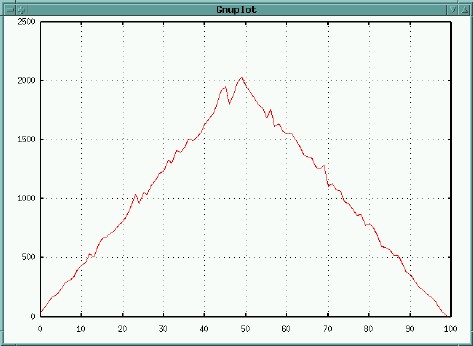
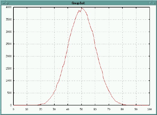
The more random() calls that you add together, the sharper the curve. This plot is the result of adding 10 random()s.

Example: a gaussian distribution lets you place objects randomly, but clustered about a center.

Uniform	Gaussian

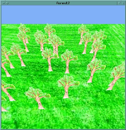
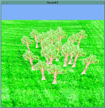
Code: forest2.cpp

next