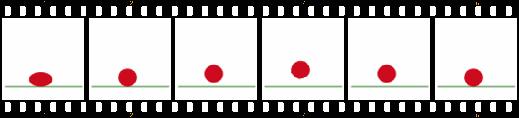
Keyframe animation uses a small sequence of key frames to define motion - all in-between frames are filled in based on the keys.
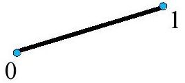
In computer animation, in-betweening is done by interpolation (linear or cubic)
Positions, rotation angles, scales, and other parameters can be interpolated.
Defined by 4 points.
Connects the first and last points; middle points control direction.
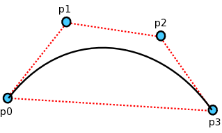
P(t) = (1 - t)3p0 + 3t(1 - t)2p1 + 3t2(1 - t)p2 + t3p3
Defined by 2 points, and tangents at those points
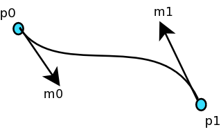
P(t) = (2t3 - 3t2 + 1)p0 + (t3 - 2t2 + t)m0 + (-2t3 + 3t2)p1 + (t3 - t2)m1
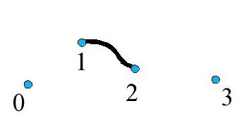
Defined by 4 points.
Curve passes through middle 2 points.
C3 = -0.5 * P0 + 1.5 * P1 - 1.5 * P2 + 0.5 * P3
C2 = P0 - 2.5 * P1 + 2.0 * P2 - 0.5 * P3
C1 = -0.5 * P0 + 0.5 * P2
C0 = P1
A cubic spline uses only 4 control values
In many cases, we have more points that we want to connect with a single curve
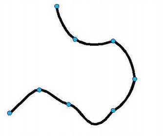
A longer curve can be broken up into multiple pieces
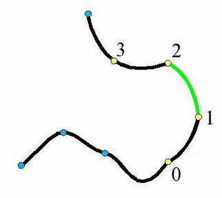
Each piece is a spline connecting 2 points, using the 4 surrounding points as control points
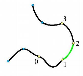
The curve parameter (t) is a measure of how far along we are in the particular segment currently being interpolated
i.e. t=0 at the beginning point (P1)
t=1 at the end point (P2)
Object motion is represented with vectors.
Velocity is a vector:
Vector direction is direction of movement
Vector magnitude is speed of movement
Velocity vector corresponds to amount object will move in one unit of time.
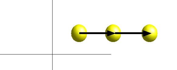
Displacement = Velocity * time
If an object starts at position P0,
with velocity V,
after t time units, its position P(t) is:
P(t) = P0 + V * t
Note: choice of units is arbitrary, as long as things are consistent.
e.g. use meters for distance, seconds for time, and meters/second for velocity.
Don't try to combine meters/second with miles/hour, for instance.
The previous formula only works if the object moves with a constant velocity.
In many cases, objects' velocities change over time.
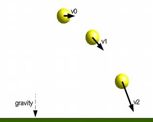
In such a case, velocity is a function that we integrate.
Displacement = 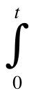 Velocity dt
In complex motion, there isn't an analytical solution (i.e. a simple formula).
Euler integration approximates an integral by step-wise addition.
At each time step, we move the object in a straight line using the current velocity:
    dt = t1 - t0
    P(t1) = P(t0) + V * dt
Velocity is the integral of acceleration:
Acceleration dt
Applying Euler integration again gives:
    dt = t1 - t0
    Acc = computeAcceleration()
    Vel = Vel + Acc * dt
    Pos = Pos + Vel * dt
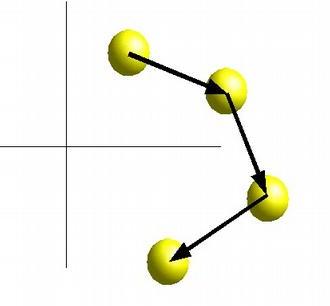
Gravity near the Earth's surface produces a constant acceleration of 9.8 m/sec2
In this case:
Acc = Vector([0, -9.8, 0])
Example: gravbounce.py
Newton's 2nd Law of Motion:
Which can be rewritten as
If an object has mass M, and force F is applied to it,
its motion can be calculated via Euler integration:
    Acc = F / M
    Vel += Acc * dt
    Pos += Vel * dt
Note that F, Acc, Vel, and Pos are all vectors. M is a scalar.
F = (G * M1 * M2) / d2
For a complete simulation, we need to calculate the force on each object every frame.
When multiple forces are applied, their vectors are added.
Example: gravorbit.py
Drag (slow moving objects):
F = Cdrag * V
Drag (fast moving objects):
F = Cdrag * V2
Buoyancy:
F = ρliquid * g * Volume
Example: buoyancy.py
